Characterizing Overconfident Failure in LLM-Based Code Generation
Abstract
Large language models (LLMs) are increasingly used for automated code generation, but generated programs can appear syntactically plausible while still failing executionbased correctness checks. Existing validation methods, such as
testing and program analysis, remain essential but are often incomplete, costly, or applied only after generation. Modelderived uncertainty is therefore a natural early reliability signal.
This paper studies the dilemma of overconfidence in code LLMs where incorrect programs are often generated with tokenlevel confidence comparable to correct programs. We study
this dilemma across four open-source code models and three execution-based benchmarks. Our analysis begins by investigating whether existing uncertainty metrics provide reliable
proxies for execution correctness in code generation. We then characterize overconfidence at both global and local token levels, asking whether incorrect programs remain indistinguishable
from correct ones under confidence and entropy summaries. Finally, we evaluate whether common mitigation strategies reduce
this failure mode, and we examine latent representations as exploratory evidence for future reliability mechanisms.
Our study yields four findings. First, existing uncertainty signals provide unstable estimates of execution failure. Second,
overconfidence is visible during generation, where failing programs often receive confidence and entropy profiles similar to passing programs. Third, local token analysis does not resolve the
issue because the most uncertain regions still provide inconsistent failure signals. Fourth, inference-time remedies improve isolated
aspects of reliability control but do not eliminate the confidence–failure mismatch. Our exploratory latent analysis suggests that
hidden representations may encode correctness-related signals that output confidence does not expose. Together, these findings identify overconfident failure as a software-engineering reliability
problem and offer a practical path toward building more reliable LLM-driven code-generation systems.
Adaptive Abstention for Reliable Code Generation
Problem. Code generators often emit syntactically valid but semantically incorrect programs when
uncertainty rises mid-generation. Post-hoc rejection detects errors after the fact, but still wastes compute and
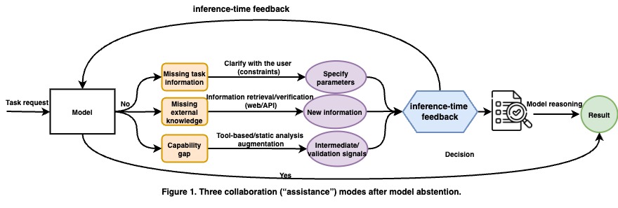
exposes users to low-quality drafts. In this section, we provide a concise overview of adaptive abstention (Figure 1),
emphasizing how it can inspire future research directions and motivate researchers to explore new avenues for
improving reliability and decision-making.
Definition.Adaptive abstention is an inference-time control policy that halts or defers
generation when a calibrated risk estimator signals insufficient reliability. Intervention occurs either
(i) pre-fill i.e., before decoding any tokens or (ii) during decoding i.e., at token/block boundaries—thereby
preventing low-quality code from being produced.
Inference-time feedback loop. When reliability is low, the system routes to clarification, retrieval/verification,
or tool/static-analysis augmentation before deciding to resume or abstain.
Pipeline: from signals to decisions
Let x be the task, yt the partial hypothesis after decoding step t, and
r̂(x, t) a calibrated risk estimate derived from logit-space features (e.g., energy, top-2 margin,
MSP), decoding dynamics, and external validation signals. Two gates implement early stopping:
Pre-fill gate (t = 0). Compute r̂(x,0) from the model’s pre-fill logits and prompt diagnostics.
If r̂(x,0) > τprefill, suspend decoding and trigger a clarification action
(missing constraints, I/O formats) via a structured query to the user. Otherwise, proceed to decoding.
Decode-time gate (token/block boundary t > 0). Maintain a running estimate
r̂(x,t) that aggregates: (a) logit-space risk; (b) decoding instability (likelihood dips, entropy spikes,
self-consistency disagreement); and (c) validation signals from lightweight tooling
(signature/schema checks, lints, static analysis, property tests). If r̂(x,t) > τdecode, pause generation
and dispatch assistance actions; resume only if risk falls below threshold after assistance.
Assistance actions and MCP integration
Assistance actions are executed through MCP-compliant tool calls (Model Context Protocol) to ensure
standardized invocation, auditing, and reproducibility:
Clarify: structured questions to the user to obtain missing task parameters.
Retrieve/verify: constrained web/API lookups for API docs, version constraints, or examples; responses are
scored and fused into r̂(x,t).
Tool/static-analysis augmentation: lints, type checks, import resolution, and sandboxed property tests that yield
intermediate pass/fail signals appended to the risk feature vector.
The decision policy π minimizes expected risk under a coverage constraint:
π = argminπ 𝔼[ risk(y) · 𝟙{emit} + cabs · 𝟙{abstain} ]
subject to 𝔼[𝟙{emit}] ≥ κ, where κ is target coverage and cabs is the abstention cost.
Thresholds τprefill and τdecode are selected to satisfy the global coverage while maximizing selective accuracy.
Scientific specification of the risk estimator
The estimator concatenates three families of features:
(F1) Logit-space = {energy, top-2 margin, MSP} possibly with class-conditional calibration;
(F2) Dynamics = {negative log-likelihood trend, entropy slope, self-consistency variance};
(F3) Validation = {lint/type-check pass rate, signature conformity, property-test outcomes, retrieval coverage}.
A lightweight logistic model g(·) (per predicted class) yields r̂(x,t) = g([F1,F2,F3]).
Preliminary Design Strategy — Key Takeaway
Implement two calibrated gates:pre-fill and decode-time are driven by a class-conditional risk estimator
that fuses logit, dynamic, and validation signals. On high risk:
(1) elicit missing constraints; (2) perform MCP-mediated retrieval/verification; (3) invoke static checks
and property tests. Resume decoding only if risk falls below the gate; otherwise emit a structured abstention
with the missing information and next steps. This policy reduces error exposure and compute waste while
preserving target coverage and improving selective accuracy.
Accuracy–Coverage Curves and Their Interpretation
Definition. The accuracy–coverage curve (a.k.a. risk–coverage curve) evaluates selective prediction.
Let the base classifier attain accuracy Accbase when all predictions are accepted
(coverage = 1.0). For a target coverage κ ∈ [0,1], keep only the top κ·N examples ranked by a
confidence score (abstain on the rest). Measure selective accuracy on this accepted subset as
Accsel(κ), and define risk as Risk(κ) = 1 − Accsel(κ).
Expected behavior across coverage levels
Full coverage (κ = 1.0).Accsel(1.0) = Accbase; risk equals the raw error rate.
Decreasing coverage. Removing low-confidence items should monotonically increase
Accsel(κ) and decrease Risk(κ) if the ranking correlates with correctness.
Low coverage regime. For small κ (e.g., < 0.3), well-ranked scores should yield
near-perfect accuracy (risk → 0). Non-monotonicity indicates poor ranking power.
Implications for our evaluation
The tables below report selective accuracy and risk for target coverages from 10% to 100%.
Overall, we expect accuracy↑ and risk↓ as coverage↓. In our results, MSP
most consistently matches this monotonic trend across settings, reflecting strong confidence–correctness alignment.
Per-model observation (e.g: DeepSeek). For the DeepSeek model, multiple
information-theoretic approaches also exhibit the desired monotone behavior, and several
variance-based techniques follow reasonably good trends as well. This suggests that DeepSeek’s scoring geometry yields higher ranking fidelity for
both confidence magnitudes and dispersion cues than other models evaluated.
Results of Accuracy-Risk Ratios Before Calibration
Calibration Approaches and Their Effects
Calibration objective. Post-hoc calibration adjusts raw uncertainty scores so that predicted
probabilities better align with empirical correctness likelihood. We evaluate two standard approaches:
Platt scaling – logistic regression mapping from raw scores to calibrated probabilities.
Isotonic regression – a non-parametric monotone mapping that preserves rank order but allows
flexible re-scaling.
Observed results
Calibration leads to modest improvements in probability quality: the Brier score decreases by
approximately 0.02–0.15% across models and datasets. However, absolute values remain high (0.2 above in most cases), indicating that
confidence calibration is still challenging in code generation tasks.
Selective performance metrics like selective accuracy and risk across coverage remain largely comparable to
pre-calibration values. MSP continues to perform robustly in all settings, with its ranking
power largely unaffected by calibration adjustments.
Model-specific behavior
For DeepSeek models, alternative uncertainty metrics show slightly different responses:
perplexity and entropy exhibit some improvements in the low-coverage regime after calibration,
reflecting better discrimination of easy versus hard instances. These gains, however, are not sufficient to
surpass the overall stability of MSP, which remains the strongest baseline across all experiments.
Results of Accuracy-Risk Ratios After Calibration
Post-Hoc Reliability Enhancements
We implement two lightweight, model-agnostic procedures operating on MSP and binary correctness only.
1) Task-Specific Weighted Platt Calibration
We transform each item’s MSP into a calibrated correctness probability using a
two-parameter logistic map. The fitting objective up-weights mispredictions so the calibrated probabilities
remain conservative when the raw score is confidently wrong. Estimation is performed out-of-fold to avoid
optimistic bias.
Inputs & Mapping
Inputs: MSP ∈ [0,1] and correctness label y ∈ {0,1}.
Mapping:p = sigmoid(a * MSP + b) (monotone; preserves ranking).
Asymmetry: errors receive higher weight to penalize overconfident mistakes.
Loss (asymmetric NLL)
Given items i = 1..N, score s_i = MSP_i, label y_i ∈ {0,1}
Weights: w(y_i) = 1 if y_i = 1
= λ ≥ 1 if y_i = 0
Minimize:
L(a,b) = (1/N) Σ_i w(y_i) * [ - y_i * log p_i - (1 - y_i) * log(1 - p_i) ]
where p_i = sigmoid(a * s_i + b)
Estimation (OOF)
Use K-fold CV. For each fold k, fit (a,b) on K−1 folds and produce probabilities for the held-out fold.
Concatenate all folds → out-of-fold calibrated probabilities for every item.
This approach:
Repairs probability scale while preserving MSP ordering.
Directly reduces overconfident assignments on errors (λ > 1).
Training-free; applicable to any single confidence score.
2) Confidence-Profiled Acceptance Policy
Using only the calibrated probability, we derive an empirical reliability profile that links confidence to error rate.
Decisions are then made by traversing from high to low confidence while monitoring cumulative error, with optional
partial acceptance in a boundary region to satisfy a target risk.
Profile Construction (OOF)
Bin scores: partition confidence [0,1] into B bins on the outer-train folds.
Estimate error: compute per-bin empirical error; assign these rates to the held-out fold.
Monotone smoothing: enforce non-increasing error as confidence rises (cumulative minimum or isotonic).
Risk-Constrained Acceptance
Inputs: calibrated p_i, bin-level error estimates r_hat(b), risk target ρ ∈ [0,1]
Procedure:
  1) Sort bins from high → low confidence.
  2) Accept entire bin if new cumulative risk ≤ ρ.
  3) If the next bin would exceed ρ, accept only the highest-p items within that bin
     until the bound is met; reject all lower bins.
Order Score for Curves
For risk–coverage curves without fixing ρ, define an order score:
q = − local_error_estimate(p) + ε·p (tiny ε to break ties).
Sorting by q yields a reliability-aware ordering for
selective accuracy/risk at chosen coverages.
Design Rationale
Decisions reflect the model’s observed reliability across confidence levels.
Out-of-fold estimates prevent leakage when building the profile.
Partial acceptance gives fine-grained control of accuracy–coverage trade-offs.
No extra annotations, logits, or top-2 margins required.
Pseudocode (Click to Expand)
Weighted Platt (OOF)
for each fold k:
    fit (a,b) on MSP,y from all folds except k using asymmetric NLL (λ on errors)
    produce p for items in fold k via p = sigmoid(a * MSP + b)
concatenate p across folds → calibrated probabilities
Confidence-Profiled Policy
for each fold k:
    on training folds: bin p, compute error per bin, enforce monotonicity
    on held-out fold: assign local error estimates r_hat by bin

Ordering for curves:
    q = − r_hat + ε·p

Risk-targeted decision:
    accept bins top-down while cumulative risk ≤ ρ
    partially accept boundary bin if needed